A Sight-Reduction Method proposed by R. Doniol
|
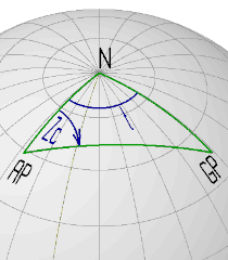
Sight Reduction is the process of solving the Navigational Triangle
for an Assumed Position and the position of an observed Celestial Body
in order to obtain a Line-of-Position.
The basic underlying problem is solving the trigonometric relations
of a spherical triangle. Since this problem arises not only in earth-bound
navigation but in a variety of fields such as astronomy and geodesy, it has
been a popular research topic for mathematicians for centuries and
still is today.
As far as the field of navigation is concerned, effort was spent to simplify
the computational process as well as to minimize the size of the required
pre-compiled data, mostly organized as look-up Tables.
In 1955, Robert Doniol published a Sight-Reduction Method, which requires
only two short and compact (single-page) Tables.
The proposed method does not directly lead to a simpler calculation scheme,
but the work inspired others to elaborate an "all-haversine-scheme" for both the
Altitude and the Azimuth, which will be described in another section.
This section will explain the background and the practical use of the
Doniol scheme for Sight Reduction.
|
Reformulating the Solutions for the Navigational Triangle
The standard "Law-of-Cosines" Altitude solution of the navigational triangle is not
very well suited for elaborating a lean and simple calculation scheme:
sin(Hc) = sin(Lat)*sin(Dec) + cos(Lat)*cos(Dec)*cos(LHA)
Besides sine and cosine table lookups, the above formula requires three time consuming and
error prone multiplication operations. This by far suitable for paper and pencil work.
Many alternative schemes have been developed since early 1800 to reformulate the
standard solution e.g. using haversine functions:
Hvers(x) = (1 - cos(x))/2 = sin2(x/2)
(note that Hvers(x) is always positive).
The Law-of-Haversine for the navigational triangle as formulated by Davis:
Hvers(Hc) = Hvers(Lat-Dec) + cos(Lat)*cos(Dec)*Hvers(t)
With t being the Meridian Angle.
This formulation has no real benefit over the previous formula, but it can
be further modified to reduce the number of multiplications or to reduce the
size of the pre-compiled Tables.
In 1955, Robert Doniol published a Sight-Reduction Method, which requires
only two single-sided Tables.
The proposed Altitude and Azimuth calculations are:
  sin(Hc) = cos(Lat-Dec) - [ cos(Lat-Dec) + cos(Lat+Dec) ] * Hvers(t)

  tan(Zc) = cos(Dec) / (f * ΔM + f' * ΔN)
Again, t is the Meridian Angle. The values for f, f', ΔM and ΔN
are determined from the two compact Tables.
When Robert Doniol published his Sight Reduction solution, he also worked out
a calculation scheme and two Tables that where conceived to be used with his
proposed method. Besides the number of recorded data, Doniol had also optimized
the numerical precision of the values in order to minimize the size of the
Tables. A reconstruction of these Tables is available
here.
The original Tables can be found from the links in the section "Sources" below.
The Tables
The first of the two tables, "Table-A", basically consists of
a record of the cosine and tangens functions. The cosine is tabulated for an
input range of 0° to 90°, the tangens function for 45° to 90°.
The angle resolution is half of a degree, resulting in about 180 record points.
The column "delta" gives the variation of the cosine value for a one-minute
change in the degree argument. This can be used e.g. for interpolation,
but these values are also part of the Azimuth calculation
(see ΔM and ΔN above).
The second table, "Table-B", is a tabulated list of the haversine function.
The column "Pa" is the angle recorded as hour-angle in time units, and the
column "a" is the corresponding haversine value
(a = Hvers(Pa)). The table is used
with the Meridian Angle as argument and has an input range of 00h to 12h
(however, in a non-equidistant scheme). Besides the haversine function,
two additional functions are listed:
f = sin2(Pa/2) / (sin(Pa) * sin(1'))
and
f'= cos2(Pa/2) / (sin(Pa) * sin(1')),
which are used in the Azimuth calculation.
Remark on the scaling factors in the tables:
The cosine- and Δ-values in Table-A, are tabulated with a scaling factor of 100000.
Whereas, the f and f' from Table-B, are tabulated with a scaling factor of 0.01.
So, the residual scaling factor for tan(Zc) using the numbers as they appear in the
Doniol Tables, is 1/100.
In the calculation scheme, Doniol accounts for this by simply omitting the last two
digits of the tabulated cos(Dec) value.
Calculation
As a first step in his calculation scheme, Doniol introduced some intermediate variables,
which are pre-evaluated:
  m = cos(Lat+Dec)  and  M=(Lat+Dec)
  n = cos(Lat-Dec)  and  N=(Lat-Dec)
  a = Hvers(t)
  γ = f * ΔM + f' * ΔN
With these variables, the Altitude / Azimuth scheme is modified to:
  sin(Hc) = n - [ n + m ] * a

  tan(Z ) = cos(Dec) / γ
As with most of the Sight-Reduction schemes, which depend on using the arc-tangens
function for the Azimuth calculation, an additional set of rules is required to obtain
the true Azimuth Angle "Zc", that refers to the upper branch of the observer's local
Meridian (the true North direction). The set of rules that are applicable for the
methode described here, are discussed further below.
Also notice, that the Doniol Tables have no tangens values for the range 0° to 45°.
So, depending on the constellation of observer's location and the position of the celestial
object, the Azimuth calulation may have to be done using the
arc-cotangens
function:
cot(Z ) = γ / cos(Dec)
Choice of the Assumed Position
To further reduce the calculation effort, Doniol's Sight-Reduction process
starts with the appropiate choice of an Assumed Position, similar to the
process that is used for appying the popular HO-249 Tables.
The Latitude for the Assumed Position is chosen such that the one of
two values M=(Lat-Dec) or N=(Lat+Dec) are on the half-degree grid as used in the
Table-A. This way only one interpolation in the cosine table is required.
Similar, for the value of the Meridian Angle t:
the Estimated Longitude is slightly adapted to obtain a Meridian Angle
value, which is ready available in the Table-B.
Rules for the Azimuth calculation
For the calculation of γ = f*ΔM + f'*ΔN, all components are
positive except for ΔM, which will be negative if |Lat| > |Dec|
(with |x| the absolute value of x).
Further, the following process may be used to calculate the true Azimuth, Zc, from the
result Z obtained from the arc-tangens function: Z = atan(cos(Dec)/γ). Z as obtained
from the Table-A, will be in the range 0° to 90°.
There are four possible schemes for the final Zc calculation:
  Zc  =        Z  =                          ___°__     (scheme 1)
  Zc  = 180° + Z  = 180° 00'  + ________  =  ___°__     (scheme 2)
  Zc  = 180° - Z  = 179° 60'  - ________  =  ___°__     (scheme 3)
  Zc  = 360° - Z  = 359° 60'  - ________  =  ___°__     (scheme 4)
If the conventional sign scheme for Latitude, Longitude and the Meridian Angle "t"
is used (positive for North and East, negative for South and West),
the following scheme selection process may be used:
 1. if the arithmetic difference N=(Lat-Dec) has the opposite sign of γ
    then use scheme 1 if t is positive
      or use scheme 4 if t is negative

 2. if the arithmetic difference N=(Lat-Dec) has the same sign as γ
    then use scheme 3 if t is positive
      or use scheme 2 if t is negative
Note, that in his publication, Doniol uses the sign of "tan(Z)" instead of the sign
of "γ", but since the value of cos(Dec) is always positive, the signs of "tan(Z)"
and "γ" are the same.
Examples
In the following section, some examples of Sight Reduction
using the Doniol scheme are elaborated.
The examples cover typical combinations of Assumed Position (N/S),
Declination (N/S) and Meridian Angles.
Example 1
This is the first example that R. Doniol used in the 1955 publication. The Meridian
Angle is given in time units: 06h 45m 37s East,
which corresponds to a degree value of 101° 24'3 (E).
 | |
EP:  LatEP =  +59° 03'0 (N)          GP: Dec =  +52° 35'0 (N)
     LonEP = -027° 33'0 (W)                t =  101° 24'3 (E)
                                               (06h 45m 37s)

     The Assumed Latitude is chosen such that the difference
     (LatAP - Dec) is on the half-degree grid of Table-A, and
     the Assumed Longitude is chosen such that a Meridian
     Angle t of 06h 46m 09s is obtained, which is available
     in Table-B (column "Pa").

AP:  LatAP =  +59° 05'0 (N)          GP: Dec =  +52° 35'0 (N)
     LonAP = -027° 41'0 (W)                t =  101° 32'3 (E)
                                               (06h 46m 09s)

     With these values, the following intermediate variables
     are calculated (with interpolation from Table-A):

     m = cos(LatAP + Dec) = cos(111°40'0) = -36920 (interp.)
     n = cos(LatAP - Dec) = cos(006°30'0) =  99357
     Σ = m + n                            =  62437

     a = 0.600           (from Table-B with Pa = "06 46 37")
     a * Σ   =                               37463

     sin(Hc) =  n - Σ * a = 99357 - 37463 =  61895
         Hc  = 38° 14'4    (with interpolation from Table-A)

     For the Azimuth, first the γ-value must be elaborated:
     γ = f * ΔM + f' * ΔN, with the values f and f' taken
     from Table-B and the Δ-values from Table-A.

     Acquiring the data for the calculation of γ:

     f = 21.1 / f'= 14.0      (Table-B with Pa = "06 46 37")

     According to the sign rules, ΔM is negative:
     ΔM = -27.1      (Table-A argument 111°30' col. "delta")
     ΔN =   3.3      (Table-A argument   6°30' col. "delta")

     γ = f * ΔM + f' * ΔN = -525

     So finally, for the Azimuth:

     cos(Dec) = 60876            (Table-A argument  52°35'0)

     tan(Z ) = cos(Dec)/γ = 608/-525 = -1.16
         Z   = 49° 15'    (with interpolation from Table-A)
         Zc  = 49° 15'    (N>0, γ<0 and t>0, so use scheme 1)
|
|
Slightly different values are obtained when solving the navigational triangle
(for the assumed position) with an electronic calculator:
Hc = 38° 14'4 and
Zc = 049° 21'0.
|
Example 2
This is the other example that R. Doniol used in the 1955 publication.
It treats a case in which the Azimuth must be calculated with the co-tangens formula.
Note that the Meridian Angle for the Assumed Position used in the original example of Doniol
(00h 58m 04s) is not in the Table-B, so a
different Assumed Longitude is used here to obtain a Meridian Angle of
00h 56m 17s, which is available from the Table-B.
 | |
EP:  LatEP =  -07° 45'0 (S)          GP: Dec =  +13° 17'0 (N)
     LonEP = -018° 30'2 (W)                t = -014° 03'8 (W)
                                               (00h 56 15s)

     The Assumed Latitude is chosen such that the sum
     (LatAP + Dec) is on the half-degree grid of Table-A, and
     the Assumed Longitude is chosen such that a Meridian
     Angle t of 00h 56m 17s is obtained, which is available
     from Table-B (column "Pa").

AP:  LatAP =  -07° 47'0 (S)          GP: Dec =  +13° 17'0 (N)
     LonAP = -018° 29'8 (W)                t =  -14° 04'2 (W)
                                               (00h 56m 17s)

     With these values, the following intermediate variables
     are calculated (with interpolation from Table-A):

     m = cos(LatAP + Dec) = cos(  5°30'0) =  99540
     n = cos(LatAP - Dec) = cos(-21°03'9) =  93317 (interp.)
     Σ = m + n                            = 192857

     a = 0.015           (from Table-B with Pa = "00 56 17")
     a * Σ   =                                2893

     sin(Hc) =  n - Σ * a = 93317 -  2893 =  90424
         Hc  = 64° 43'2    (with interpolation from Table-A)

     Acquiring the data for the calculation of γ:

     f =  2.1 / f'= 139.      (Table-B with Pa = "00 56 17")

     ΔM =   2.8      (Table-A argument   5°30' col. "delta")
     ΔN =  10.4      (Table-A argument  21°00' col. "delta")

     γ = f * ΔM + f' * ΔN = 1451

     So finally, for the Azimuth:

     cos(Dec) = 97333            (Table-A argument  13°17'0)

     Since γ (1451) is larger than the value to be used for
     cos(Dec) (973), the co-tangens formula will be used:

     cot(Z ) = γ/cos(Dec) = 1451/973 = 1.49
         Z   =  33° 50'    (with interpolation from Table-A)
         Zc  = 326° 10'    (N<0, γ>0 and t<0, so use scheme 4)
|
|
Almost the same values are obtained when solving the navigational triangle
(for the assumed position) with an electronic calculator:
Hc = 64° 43'3 and
Zc = 326° 24'0.
|
Example 3
 | |
EP:  LatEP =   31° 01'3 (N)          GP: Dec =  -10° 12'6 (S)
     LonEP =  014° 50'4 (W)                t = -051° 40'0 (W)
                                               (03h 26m 40s)

     The Assumed Latitude is chosen such that the sum
     (LatAP + Dec) is on the half-degree grid of Table-A, and
     the Assumed Longitude is chosen such that a Meridian
     Angle t of 03h 26m 44s is obtained, which is available
     from Table-B (column "Pa").

AP:  LatAP =   31° 12'6 (N)          GP: Dec =  -10° 12'6 (S)
     LonAP = -030° 00'0 (W)                t = -051° 41'0 (W)
                                               (03h 26m 44s)

     With these values, the following intermediate variables
     are calculated (without any interpolation from Table-A):

     m = cos(LatAP + Dec) = cos( 21°00'0) =  93358
     n = cos(LatAP - Dec) = cos( 41°25'2) =  74989
     Σ = m + n                            = 168347

     a = 0.190            (from Table-B with Pa = "03 26 44")
     a * Σ   =                               31986

     sin(Hc) =  n - Σ * a = 74989 - 31986 =  43003
         Hc  = 25° 28'2     (with interpolation from Table-A)

     Acquiring the data for the calculation of γ:

     f = 8.3 / f'=  35.5       (Table-B with Pa = "03 26 44")

     According to the sign rules, ΔM is negative:
     ΔM = -10.0       (Table-A argument  21°00' col. "delta")
     ΔN =  19.3       (Table-A argument  41°30' col. "delta")

     γ = f * ΔM + f' * ΔN =  598

     and finally, for the Azimuth:

     cos(Dec) = 98545             (Table-A argument  10°12'6)

     tan(Z ) = cos(Dec)/γ = 985/598 = 1.64
         Z   =  58° 45'    (with interpolation from Table-A)
         Zc  = 238° 45'    (N>0, γ>0 and t<0, so use scheme 3)
|
|
The following values are obtained when solving the oblique triangle with
an electronic calculator:
Hc = 25° 28'1 and
Zc = 238° 48'0.
|
Example 4
 | |
EP:  LatEP =   30° 12'0 (N)          GP: Dec =  -10° 12'0 (S)
     LonEP = -030° 12'0 (W)                t =  040° 12'0 (E)
                                               (02h 40m 48s)

     The Easimated Latitude is already such that the sum
     (LatAP + Dec) is on the half-degree grid of Table-A, and
     the Assumed Longitude is chosen such that a Meridian
     Angle t of 02h 42m 09s is obtained, which is available
     from Table-B (column "Pa").

AP:  LatAP =   30° 12'0 (N)          GP: Dec =  -10° 00'0 (N)
     LonAP = -030° 32'1 (W)                t =  040° 32'3 (W)
                                               (02h 42m 09s)

     With these values, the following intermediate variables
     are calculated (without any interpolation from Table-A):

     m = cos(LatAP + Dec) = cos( 20°00'0) =  93969
     n = cos(LatAP - Dec) = cos( 40°24'0) =  76154
     Σ = m + n                            = 170123

     a = 0.120            (from Table-B with Pa = "02 40 09")
     a * Σ   =                               20415

     sin(Hc) =  n - Σ * a = 76154 - 20415 =  55740
         Hc  = 33° 52'6     (with interpolation from Table-A)

     Acquiring the data for the calculation of γ:

     f = 6.3 / f'=  47        (Table-B with Pa = "02 40 09")

     According to the sign rules, ΔM is negative:
     ΔM =  -9.9       (Table-A argument  20°00' col. "delta")
     ΔN =  18.9       (Table-A argument  40°30' col. "delta")

     γ = f * ΔM + f' * ΔN = 817

     and finally, for the Azimuth:

     cos(Dec) = 98542             (Table-A argument  10°12'0)

     tan(Z ) = cos(Dec)/γ = 985/817 = 1.21
         Z   =  50° 30'
         Zc  = 129° 30'    (N>0, γ>0 and t>0, so use scheme 2)
|
|
The following values are obtained when solving the navigational triangle
(for the assumed position) with an electronic calculator:
Hc = 33° 52'5 and
Zc = 129° 36'.
|
Discussion
The beauty of the Doniol method for Sight-Reduction, clearly lies in the compact size
of the tables that can be used with this scheme. And this comes without any significant
loss of accuracy for the calculated Altitude and Azimuth.
The downside is the rather complex calculation scheme. If the method is used without
electronic calculator, the required multiplications and divisions must be performed
manually using paper and pencil.
A note on the accuracy of the presented Sight-Reduction Methode: I have
performed an error evaluation for the determination of Altitude and Azimuth,
using the above method and comparing the results with a straight solution of
the trigonometric equations for Altitude and Azimuth.
For this, about two milion different cases were analyzed, which were chosen
randomly, but with an equal spreading over the two resulting variables
Altitude and Azimuth.
The statistical results can be summerized as follows: the maximum error on the
Altitude is smaller than 1.5 minutes for all analyzed cases, wheras the maximum
error for the Azimuth can be as large as 10 degrees.
However, if cases in which the Altitude is larger than 80 degrees are ommited,
the Azimuth error is smaller than 2 degrees.
So, it should be taken ito account that the presented method may not always perform
well in terms of Azimuth accuracy, if the location of the observer is near to the
Geographical Position of the Celestial Object.
Sights done under such conditions may not always be avoidable, but it should
be kept in mind that the result for the Azimuth may not be as accurate as expected.
Sources
|