The Conformal Mercator Projection
Map projections are attempts to portray the surface of the earth or a portion
of the earth on a flat surface. Some distortions of conformity, distance,
direction, scale, and area always result from this process. Some projections
minimize distortions in some of these properties at the expense of maximizing
errors in others. Other projection are attempts to only moderately distort
all of these properties.
A map projection is conformal if the angles in the original features
are preserved in the image on the chart. Over small areas the shapes of
objects will be preserved. A line with constant orientation (a rhumb line
or loxodrome) will be straight on a conformal projection.
On a conformal projection, the scale is constant in all directions
about each point but scale varies from point to point on the map.
For practical nautical navigation only the conformal Mercator projection
is of interest. This projection is still used today for nautical charts.
The projection was developed by Gerardus Mercator in 1569 as an aid to
navigation. It has the special property that loxodromes or rhumb
lines are represented as straight lines on the map, which has a fundamental
impact upon practical navigation.
The gnomonic projection on the other hand, has the property that
great circles appear as straight lines, making it easy to plot the shortest
route between two points. Transferred to the Mercator projection, the great
circle route will appear as a curved line that can be approximated by straight-line
segments. The straight-line segments on the Mercator projection are easier
to follow since this only requires following a constant compass direction.
History
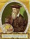 The "Mercator Projection" is named after the Flemish cartographer Gerard
Kremer (1512-1594) , who later adopted the latin name Gerardus Mercator.
He published the first maps using his new developed projection in 1569,
but only in the beginning of the 17th century, after 1599 when Edward Wright
published a detailed explanation of the technique Mercator used, the conformal
Mercator Projection became popular among nautical cartographers.
The "Mercator Projection" is named after the Flemish cartographer Gerard
Kremer (1512-1594) , who later adopted the latin name Gerardus Mercator.
He published the first maps using his new developed projection in 1569,
but only in the beginning of the 17th century, after 1599 when Edward Wright
published a detailed explanation of the technique Mercator used, the conformal
Mercator Projection became popular among nautical cartographers.
The interesting fact of the Mercator Projection is that the underlying
mathematical framework including logarithms (developed by Napier around
1610) calculus (developed by Leibnitz and Newton around 1660) and differential
geometry (developed by Gauss around 1800) was not yet available at the time
Mercator developed the techniques for his conformal projection.
The conformal Projection
In the 16th century, trading over the new discovered seaways had developed
to an important economical factor in western Europe. The compass was the
principal navigation instrument and navigation itself was based on dead
reckoning. Therefore, it was most convenient to sail tracks of constant
heading or sailing along a loxodrome.
With the rapid expansion of sea trading, cartography flourished
from the increasingly detailed geographical information. Cartographers
not only had to deal with the increasing amount of new data, they also
had to think of how to map this data on a chart such that it could be most
practically used for sea navigation.
If loxodromes and thus the tracks sailed by the trading ships, would
be a straight lines in the nautical chart, this would simplify navigation
considerably. At the same time the contours of a coast line on the map
must provide a good image of the real coast line. And since bearings are
the basis for coastal navigation, nautical maps should also be "angle-true".
This was the problem Mercator was working on during the years around
1560. The requirement that a rhumb line must map to a straight line in
the chart, requires that the meridian lines must be mapped to parallel
lines on the chart. Together with the "angle-true"- or conformity requirement,
the basic grid of a practical nautical chart Mercator was looking for,
would consist of an orthogonal grid with meridian lines running parallel
bottom-to-top and parallel lines of constant latitude running left-to-right.
If the meridian lines are parallel lines on the chart, but converge
to the poles on the globe, the scaling factor between features on the globe
and their image on the chart, cannot be the same for all locations on the
globe. It was clear to Mercator that to obtain the required characteristics
for his practical nautical chart, the scaling factor has to increase with
the latitude. In order to obtain conformity, the latitude-depending scaling
factor of the chart must be applied in all directions for all points on
the chart. So not only the "east-west" directions will be stretched to
obtain parallel meridians, also the "north-south" directions must be scaled
with the same latitude-depending factor.
In the extreme case, the pole is subject to an infinite degree of distortion
since it will be stretched into a line having the same length as the Equator,
although it is a point on the globe. Therefore, the image of the poles
is infinitely far away from the Equator . As a consequence, the poles will
never be visible on a standard Mercator chart. But this has no further
practical implications for nautical navigators.
Although the mathematical toolbox to develop an analytical solution
to this problem did not yet exist, Mercator managed to develop "scaling
tables", with which he was able to construct nautical charts using what
we call today a "conformal Mercator projection".
Since there is no geometric projection to produce a Mercator
chart, the Mercator Projection is often illustrated as a projection from
the center of the earth on a cylinder wrapped around the equator. However,
that cylindrical projection is only an approximation of the Mercator projection
and it has not the property that Mercator was seeking: the rhumb lines
are not straight lines in a cylindrical projection. |
 |
The cylindrical projection and the Mercator projection have in common
that meridians lines and lines of parallels are straight and intersect
orthogonally. Also since the meridian lines don't converge towards the
poles (as they do on a globe), the scale of the chart must increase as
the latitude increases. The difference to the Mercator projection is that
a cylindrical projection has different horizontal and vertical scaling
factors and thus it is not conformal.
Nautical charts used today still are Mercator charts. The fact that meridians
are parallel makes it easy to measure angles such as headings and bearings from these.
But for example in aeronautics, Mercator charts are not used any more because today
aeronautic navigation is based on radio navigation.
Aircraft pilots use charts which shows great circles as straight lines.
Rhumb lines on aeronautical charts are curved lines.
Surveyors still use other charts since they are interested in accurate distance
and bearings over long distances.
The Mathematical Framework
In mathematics, a projection is a function which takes the coordinates
of a point on one surface and transforms them into the coordinates of a
point on another surface. More specific in cartography the projection function
takes a point from the surface of the globe and transforms it to a point
on a plane.
The following variables will be used in the next mathematical equations
and functions:
Lat : Latitude in degrees
Lon : Longitude in degrees

X   : east -west  distance on the chart (e.g. in mm)
Y   : north-south distance on the chart (e.g. in mm)
c   : scale of the chart (e.g. in mm/degree)
The conformal Mercator projection
An infinitesimal small square with sides (dLon, dLat) located on the globe
at longitude "Lon" and latitude "Lat" has a size on the globe of
dX  = c' * dLon * cos(Lat)
dY  = c' * dLat
with c' the scaling factor between the units of Lon/Lat (°) and the
units of X/Y (e.g. km).
However, this transformation maintains conformity only for a small range of
Latitude. Indeed, since the spacing of the meridians is not constant but depends
on the Latitude, the meridian lines will not run parallel.
To obtain parallel meridians, the following scaling must be applied:
c = c' * cos(Lat)
To obtain conformity, the scaling has to be applied for both directions X and Y:
dX  = c * dLon
dY  = c * dLat / cos(Lat)
The transformation function is obtained by integrating these differential
equations. The chart origin (X,Y) = (0,0) is mapped to location (Lon,Lat)
= (0°,0°) to resolve the "integration constant":
X   = c * Lon
Y   = c * (ln ( tan ( Lat/2 + 45°))
This is the Mercator conformal projection function, transforming an arbitrary
location on the surface of the Earth (Lon,Lat) to a point on a two dimensional
chart (X,Y). Longitudes east of the Prime Meridian have positive sign and
map to positive X values; longitudes west of the Prime Meridian map to
negative values of X. In a similar way, latitudes north of the equator
map to positive Y values; latitudes south of the equator have a negative
sign and map to negative Y values.
Notice that the above mathematical description is based on a perfect spherical
body and does not take into account the ellipticity of the Earth.
The cylindrical projection
The cylindrical projection, which is often used as geometrical illustration
of the Mercator projection has the following projection function:
X   = c * Lon
Y   = c * tan(Lat)
This cylindrical projection does not map a loxodrome to a straight line
in the chart. In a conformal Mercator projection the scaling factor c is
the same for both X and Y dimensions. The cylindrical projection has different
scaling factor for X and Y directions and thus is not conformal. This is
illustrated in the pictures below for a NW loxodrome:
Loxodrome on a globe
|
Loxodrome on a chart with a
"Mercator grid" |
Loxodrome on a chart with a
"cylinder grid" |
The cylindrical projection is nevertheless useful as an approximation
of the Mercator projection in a small plotting range (e.g. a couple of
degrees of latitude around the location of a vessel).
For small-range plotting areas a chart with an approximate Mercator
grid can be constructed as a cylindrical grid in a geometrical way as described
in "Worksheets for Lines-of-Position". These plotting sheets are used in
the practice of celestial navigation to determine the position from two
or more Lines-of-Position.
The gnomonic Projection
The conformal Mercator projection has the great advantage that rhumb lines
or loxodromes are mapped to straight lines in the chart. The gnomonic projection
produces charts in which great-circle segments are mapped as straight lines.
Since a great-circle segment is the shortest track between two points
on the globe, gnomonic charts can be advantageously used for nautical navigation
to find the shortest route between two ports.
However, the difference in distance between a rhumb line and a great-circle
segment connecting the same two points on the globe is only significant
for very large distances and higher latitudes (e.g. sailing the Viking's route
from Norway to Iceland). Moreover, with simple navigation tools, such as a compass
to fix the course, it is rather difficult to sail great-circle segments.
So for sailors, gnomonic charts have little practical value.
For aircraft traffic however, the shortest route for long-distance
flights is a time and profit issue. And since aircrafts also have sophisticated
navigation equipment on board, enabling computer controlled navigation
along great-circle segments, gnomonic charts have been very useful for
aeronautic navigation.
The gnomonic projection is a geometrical projection obtained as follows:
take a point with location (Lon_sp, Lat_sp)
in which the plane of projection is tangent with the globe. This point
is called the "standard point" or "point of tangency" for the projection.
For any point on the globe with location (Lon,Lat) construct a "projection
line" connecting this location with the center of the globe. The location
(Lon, Lat) is then mapped to the point where the corresponding "projection
line" intersects with the plane of projection.
A great circle is the intersection of a plane through the center of
the globe with the surface of the globe. All projection lines of the points
of a great circle are contained in the plane which defines the corresponding
great circle. The intersection of this plane with the plane of projection
is a straight line. Thus great circles map as straight lines for this projection.
Since the gnomonic projection maps antipodal points on the globe to
the same point on the chart, it can only be used to map one hemisphere
at a time. Only around the standard point, all major characteristics (angles,
area, distances, ...) are retained with distortions becoming radially pronounced
with increasing distance from the standard point.
The projection function to obtain a gnomonic chart is:
X   = c * ( sin(Lon - Lon_sp) * cos(Lat) ) / cos(a)
Y   = c * ( cos(Lat_sp) * sin(Lat) - sin(Lat_sp) * cos(Lat) * cos(Lon - Lon_sp) ) / cos(a)
with "a" the angular distance of the point (Lat,Lon) to the center of the
projection (Lon_sp, Lat_sp):
cos(a) = sin(Lat_sp) * sin(Lat) + cos(Lat_sp) * cos(Lat) * cos(Lon - Lon_sp)
If the location (Lon_sp,Lat_sp)
= (0°,0°) is chosen as point of tangency (standard point) the projection
function simplifies to:
X   = c * tan(Lon)
Y   = c * tan(Lat) / cos(Lon)
The principle of this gnomonic projection and the resulting chart grid
of meridian lines and parallels of constant latitude is illustrated in
the pictures below:
The example on the right shows the principle of a gnomonic projection.
The projection lines radiate from the center of the globe to the plane of projection,
which lies in front of the globe.
The point of tangency is located at Lon = 0° and
Lat = 0°.
The yellow projection lines are connected to points located on the same parallel
(N 30°). The green projection lines are related to some points located on the same meridian
(E 30°).
The blue points are located on the surface of the globe
and the red points are the corresponding intersection points with the plane
of projection on which the gnomonic image of the globe is mapped.
|
 |
Loxodrome on a chart with a
"gnomonic grid" |
The example of the loxodrome in the picture on the right also illustrates
that - even on this scale - there is no real significant difference between a loxodrome
and a great-circle segment (the loxodrome is almost a straight line).
Loxodrome distances and courses may also be calulated mathematicaly.
This may be usefull e.g. for determining the distance of long tracks
covering more than one chart. Also for determining the loxodrome course
of transatlantic journeys this mathematical approach may be usefull.
Please go to the "notes on loxodrome calculations"
to read more on this topic.
To examin the difference between loxodrome tracks and the corresponding great-circle tracks
the following interactive pages may be used:
As an example the great-circle distance across the Atlantic Ocean between
Cape Town (South Africa; 36°S 17°E) and
Montevideo (Uruguay; 37°S 56°W) is 3428 nautical miles.
The loxodrome distance is 3521 nautical miles.
So the great-circle track is about 100 nautical miles (less than 3%) shorter than the loxodrome track.
However, for ocean sailing, taking advantage of favourable winds and currents is usualy
of much more importance than sailing the shortest track.
|